The theory of monoids
In this notebook, we will construct a presentation of the theory of monoids or associative algebras in rewalt. Depending on your favourite gadget, you may see this as the data presenting a monoidal category (PRO) or an operad.
Adding the sorts and operations
Let’s first import rewalt and create an empty diagrammatic set — an object of class DiagSet — that we will call Mon.
[1]:
import rewalt

Mon = rewalt.DiagSet()
You know how a monoidal category can be seen as a one-object bicategory (its delooping)? This is how we do it in rewalt too: the sorts of a monoidal theory are 1-cells going to and from a single 0-cell.
So first of all, we add a single 0-dimensional generator to our diagrammatic set.
[2]:
pt = Mon.add('pt')
This adds a 0-dimensional generator to Mon, assigns it the name 'pt' and returns the Diagram object that “picks” that generator only; we assign this diagram to the variable pt.
Next, we add a single 1-dimensional generator, corresponding to the single sort of our theory.
[3]:
a = Mon.add('a', pt, pt)
The two extra arguments that we gave to add specify the input, or source boundary of the new generator, and the output, or target boundary of the new generator, respectively. In this case they are both equal to the unique “point”.
By the way, if you fail to assign the output of add to a variable, you can always retrieve it later by giving the generator’s name to Mon’s indexer.
[4]:
assert a == Mon['a']
There is not much that we can do with 0-cells… but with 1-cells, we can create larger diagrams by pasting.
The paste method pastes together diagrams along the k-dimensional output boundary of one and the k-dimensional input boundary of the other, when these match each other.
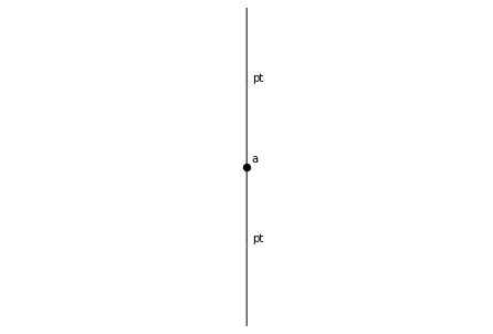
For a 1-cell, the only non-trivial boundary is the 0-dimensional one; pasting along it corresponds to “concatenation of paths”. We can concatenate a to itself as many times as we want. Let’s also visualise the result as a “1-dimensional string diagram”.
[5]:
a.draw()
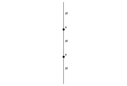
[6]:
a.paste(a).draw()
[7]:
a.paste(a).paste(a).draw()
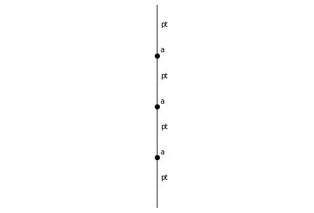
And so on. Note that paste can also take an integer argument specifying the dimension of the boundary along which to paste; it defaults to the minimum of the two diagrams’ dimensions, minus 1. In this case the minimum of 1 and 1 is 1, which minus 1 equals 0, and that’s the boundary we want.
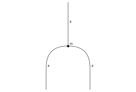
Now that we have the sorts, let’s add the operations. The monoid multiplication takes two inputs and returns one output. This corresponds to a 2-dimensional generator, whose input is a.paste(a), and output a.
[8]:
m = Mon.add('m', a.paste(a), a)
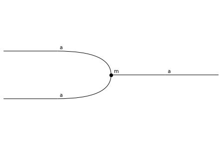
And let’s picture this as a string diagram.
[9]:
m.draw()
(As you can see, string diagrams by default go from bottom to top. If you prefer left-to-right, or top-to-bottom, or right-to-left orientation, you can pass it as an argument to draw; or to change the default setting, reassign rewalt.strdiags.DEFAULT['orientation'].)
[10]:
m.draw(orientation='lr')
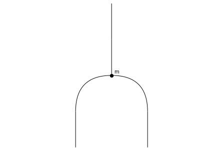
Since we have a single sort, it is a little pointless to label the wires. Same for labelling the unique point. Let’s switch labels off for these generators.
[11]:
Mon.update('a', draw_label=False)
Mon.update('pt', draw_label=False)
m.draw()
Next, we want to add the monoid unit, which is a “nullary” operation. Here things get a little more subtle.
Cells in rewalt are not allowed to have “strictly lower-dimensional” inputs or outputs: if we try to add a 2-dimensional generator whose input is a 0-dimensional diagram, we will get an error.
[12]:
try:
    u = Mon.add('u', pt, a)
except ValueError:
    print('Nope')
Nope
Instead, we have to use “weak units”, in the form of degenerate diagrams. (This may seem like a hassle in dimension 2, where “everything can be strictified”, but pays off in higher dimensions.)
A simple constructor for degenerate diagrams is the unit method, which creates a “unit diagram”, one dimension higher.
[13]:
assert pt.dim == 0
assert not pt.isdegenerate

assert pt.unit().dim == 1
assert pt.unit().isdegenerate
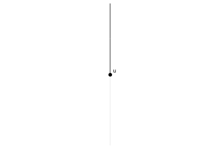
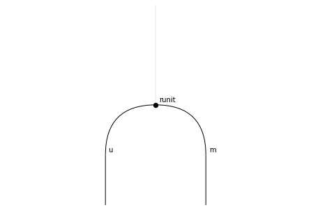
So to add the monoid unit, we make pt.unit() its input.
In string diagrams, degenerate cells are represented as translucent wires (when wires), or as “node-less nodes” (when nodes).
[14]:
u = Mon.add('u', pt.unit(), a)
u.draw()
Adding “oriented equations”
Now we can compose diagrams with paste in two directions, along the 0-boundary (“horizontally”) or the 1-boundary (“vertically”)…
[15]:
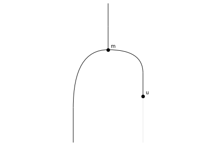
u.paste(m, 0).draw() # "horizontal" pasting
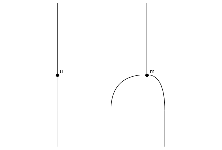
[16]:
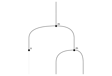
u.paste(m, 0).paste(m).draw() # ...and now "vertical" pasting
A useful alternative to paste (especially in an “operadic” setting) are the methods to_inputs and to_outputs, which allow us to paste a diagram only to some inputs and outputs of another diagram.
To use these in practice, one must know that every node and wire in a string diagram have a unique position. We can use the keyword arguments positions (both nodes and wires), nodepositions, and wirepositions to enable positions in string diagram output.
[17]:
m.draw(positions=True)
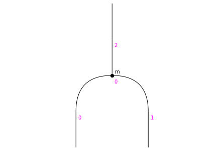
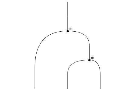
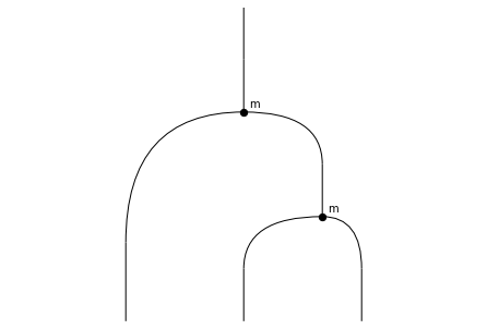
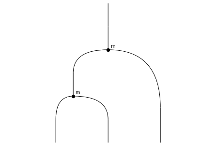
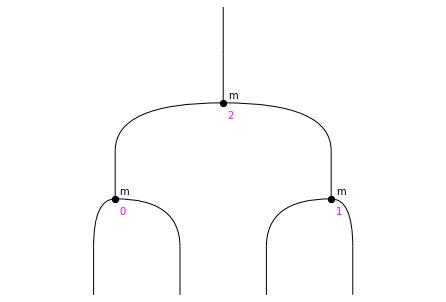
Now, we can paste another multiplication either to the input in position 0, or the input in position 1.
[18]:
m.to_inputs(0, m).draw()
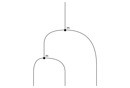
[19]:
m.to_inputs(1, m).draw()

These two diagrams happen to be the two sides of the associativity equation, so let’s add this equation to our presentation!
Or rather, we add an oriented associativity equation, or associativity rewrite, or “associator”, as a 3-dimensional generator. All the cells in diagrammatic sets have a direction.
[20]:
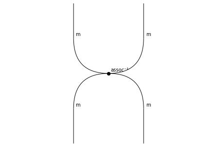
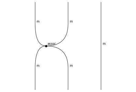
assoc = Mon.add('assoc', m.to_inputs(0, m), m.to_inputs(1, m))
assoc.draw()
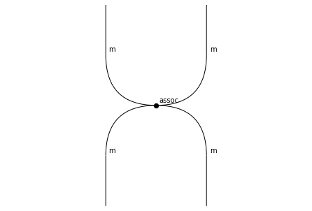
You can see that, when we draw a 3-dimensional diagram, we obtain a “2-dimensional slice” string diagram, where nodes correspond to 3-cells and wires to 2-cells. (In general, for an n-dimensional diagram, nodes are n-dimensional cells and wires are (n-1)-dimensional cells).
Here, assoc is a 3-dimensional cell that has two m 2-cells in its input, and two m 2-cells in its output.
To see the two “sides” of the rewrite, we can either use the draw_boundaries method, or first call input/output and only then draw.
[21]:
assoc.draw_boundaries()

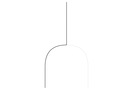
Next, let’s add left unitality and right unitality equations/rewrites. The left-hand side of the left unitality equation is this.
[22]:
m.to_inputs(0, u).draw()
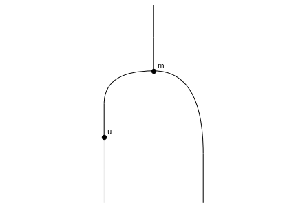
This diagram is supposed to be equal to “the identity operation” on our sort (which would be the unit on a)… but not quite, because it contains a weak unit in the input; instead we want to equate to another degenerate cell called the left unitor on a. We build it like this.
[23]:
a.lunitor('-').draw()
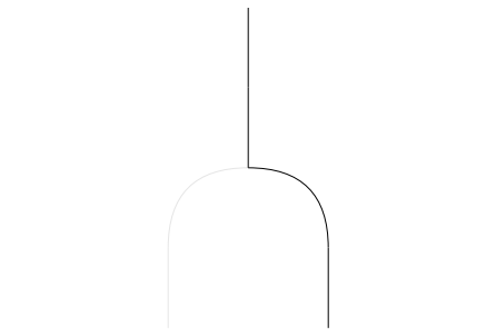
The argument '-' specifies that the unit should appear in the input, and not the output.
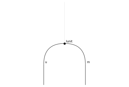
Now we can add the “left unitality” generator.
[24]:
lunit = Mon.add('lunit', m.to_inputs(0, u), a.lunitor('-'))
lunit.draw()
We proceed similarly for the “right unitality” generator.
[25]:
runit = Mon.add('runit', m.to_inputs(1, u), a.runitor('-'))
runit.draw()
runit.draw_boundaries()
Making the equations go both ways
That’s it, we now have a presentation of the theory of monoids!
Except our “equations” are really directed rewrites. What if we want to use them in both directions? Luckily, we have methods for “weakly inverting” a generator. Let’s try it on assoc.
[26]:
Mon.invert('assoc')
[26]:
(<rewalt.diagrams.Diagram at 0x7f72f7faf100>,
 <rewalt.diagrams.Diagram at 0x7f72f7faeb60>,
 <rewalt.diagrams.Diagram at 0x7f72f843f250>)
This returned 3 diagrams, which corresponds to the fact that 3 new generators were added. Let’s see what happened. We can see a list of the generators, ordered by dimension, with the DiagSet method by_dim.
[27]:
Mon.by_dim
[27]:
{0: {'pt'},
 1: {'a'},
 2: {'m', 'u'},
 3: {'assoc', 'assoc⁻¹', 'lunit', 'runit'},
 4: {'inv(assoc, assoc⁻¹)', 'inv(assoc⁻¹, assoc)'}}
So, first of all, there’s a new 3-dimensional generator, assoc⁻¹.
[28]:
Mon['assoc⁻¹'].draw()
Mon['assoc⁻¹'].draw_boundaries()
This is the “weak inverse” of assoc: a generator with the same boundaries as assoc, but going in the reverse direction. If a generator has a weak inverse, we can get it with the inverse attribute.
[29]:
assert assoc.inverse == Mon['assoc⁻¹']
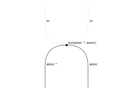
Then, we have two new 4-dimensional generators, inv(assoc, assoc⁻¹) and inv(assoc⁻¹, assoc).
[30]:
Mon['inv(assoc, assoc⁻¹)'].draw()
Mon['inv(assoc, assoc⁻¹)'].draw_boundaries()
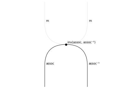
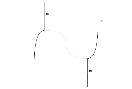
This generator “exhibits” the fact that assoc⁻¹ is a right inverse (right in diagrammatic order; left in composition order) for assoc: it goes from the pasting of assoc and assoc⁻¹, to a weak unit on the input of assoc.
We call this a right invertor for assoc, and can get it with the rinvertor attribute.
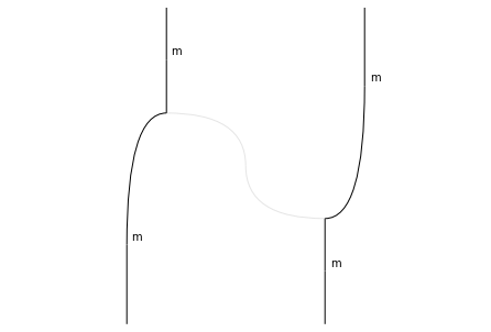
Similarly, inv(assoc, assoc⁻¹) exhibits the fact that assoc⁻¹ is a left inverse for assoc. We call this a left invertor for assoc, and can retrieve it with the linvertor attribute.
Note that the left invertor for assoc is the right invertor for assoc⁻¹, and vice versa!
[31]:
assert assoc.rinvertor == Mon['inv(assoc, assoc⁻¹)']
assert assoc.linvertor == assoc.inverse.rinvertor
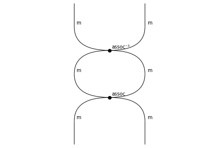
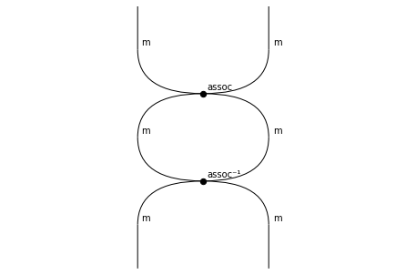
In the theory of diagrammatic sets, these two “witnesses” should, themselves, be weakly invertible cells; since this would require an infinite number of generators, we leave it to the user to invert them when/if needed.
[32]:
Mon['inv(assoc⁻¹, assoc)'].draw()
Mon['inv(assoc⁻¹, assoc)'].draw_boundaries()
Computing with diagrammatic rewrites
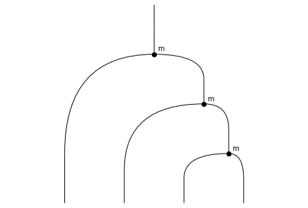
Let’s start using our presentation to make some diagrammatic computations. First, we create a 2-dimensional diagram.
[33]:
start = m.to_inputs(0, m).to_inputs(0, m)
start.draw(nodepositions=True)
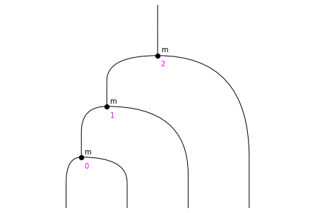
In traditional algebraic notation, this would correspond to the term \(m(m(m(x, y), z), w)\).
We see that we can apply an associativity rewrite/equation in two places, corresponding to the nodes in positions (0, 1) and to the nodes in positions (1, 2).
We can “apply rewrites” with the rewrite method. The result of rewrite is not going to be the “rewritten” 2-dimensional diagram. Instead, it will be a 3-dimensional diagram whose input is the original diagram, and output is the rewritten diagram: an “embodiment” of the rewrite operation.
(The rewrite method is, in fact, a special instance of to_outputs; once you understand the principles of higher-dimensional rewriting, you should be able to see why).
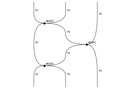
[34]:
rew1 = start.rewrite([0,1], assoc)
rew1.draw()
rew1.output.draw(nodepositions=True)
In the rewritten diagram, we can only apply assoc to the nodes (0, 2).
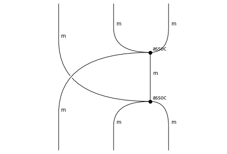
[35]:
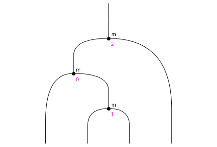
rew2 = rew1.output.rewrite([0, 2], assoc)
rew2.output.draw(nodepositions=True)
Now, we can apply assoc to the nodes (1, 2).
[36]:
rew3 = rew2.output.rewrite([1, 2], assoc)
rew3.output.draw()

We cannot apply assoc anywhere else. (Of course we could start applying assoc⁻¹).
Let’s put together our sequence of rewrites.
[37]:
seq1 = rewalt.Diagram.with_layers(rew1, rew2, rew3)
seq1.draw()

(We could have equally defined seq1 as rew1.paste(rew2).paste(rew3)).
We can use the method rewrite_steps to get all our rewrite steps… and we can even produce a little gif animation with all the steps. (We’ll make it loop backwards as well so it doesn’t end too soon.)
[38]:
rewalt.strdiags.to_gif(*seq1.rewrite_steps, loop=True, path='monoids_1.gif')
Let’s go back to the start and pick a different rewrite, the one on nodes (1, 2).
[39]:
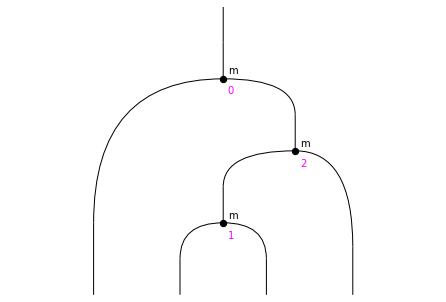
rew4 = start.rewrite([1, 2], assoc)
rew4.output.draw(nodepositions=True)
[40]:
rew5 = rew4.output.rewrite([0, 2], assoc)
rew5.output.draw()
[41]:
seq2 = rew4.paste(rew5)
seq2.draw()
rewalt.strdiags.to_gif(*seq2.rewrite_steps, loop=True, path='monoids_2.gif')


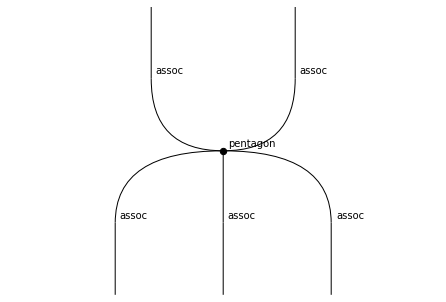
You can see that seq1 and seq2 are two different sequences of rewrites with the same starting and ending point.
If you are familiar with the characterisation of monoidal categories as pseudomonoids in the monoidal 2-category of categories with cartesian product, you may recognise the two sides of Mac Lane’s pentagon equation!
Indeed, we can add a 4-dimensional generator between the two, embodying Mac Lane’s pentagon.
[42]:
pentagon = Mon.add('pentagon', seq1, seq2)
pentagon.draw()
pentagon.draw_boundaries()
We could go on and add generators corresponding to Mac Lane’s triangle… but this was supposed to be about the theory of monoids, not of lax or pseudomonoids, so let’s stop here instead.